A Model for Control

By collecting data from real human motion our system models behavior patterns as statistical densities over configuration space. Different configurations have different observation probabilities.

One very simple behavior model is the mixture model, in which distribution is modeled as a collection of Gaussians. In this case the composite density is described by:

$$\sum_{k=1}^{N} P_k \cdot \Pr( {\bf O} \vert \lambda=k )$$ (1)

where P_k is the observed prior probability of sub-model k.

The mixture model represents a clustering of data into regions within the observation space. Since human motion evolves over time, in a complex way, it is advantageous to explicitly model temporal dependence and internal states. A Hidden Markov Model (HMM) is one way to do this, and has been shown to perform quite well recognizing human motion[19].

The probability that the model is in a certain state, S_j given a sequence of observations, ${\bf O}_{1}, {\bf O}_{2}, \ldots, {\bf O}_{N}$, is defined recursively. For two observations, the density is:

$$\Pr( {\bf O}_{1}, {\bf O}_{2}, {\bf q}_2 = S_j ) = \left[ \... ...\pi_{i} b_{i}({\bf O}_1){\bf a}_{ij} \right] b_{j}({\bf O}_2)$$ (2)

Where $\pi_{i}$ is the prior probability of being in a state i, and $b_{i} ({\bf O})$ is the probability of making the observation ${\bf O}$while in state i. This is the Forward algorithm for HMM models [16].

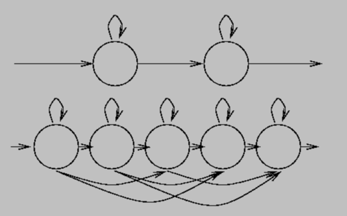
Estimation proceeds by identifying the most likely state given the current observation and the last state, and then using the observation density of that state as described above. We restrict the observation densities to be either a Gaussian or a mixture of Gaussians. There are well understood techniques for estimating the parameters of the HMM from data [16]. Figure 5 shows some representative HMM topologies.

  

Figure: Top: A typical illustration of a two state HMM. Circles represent states with associated observation probabilities, and arrows represent non-zero transition arcs, with associated probability. Bottom: This is an illustration of a five state HMM. The arcs under the state circles model the possibility that some states may be skipped.