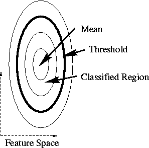
Figure A.1:
Classification is the process of sorting feature vectors into categories, or classes. Feature vectors are points in a feature space that is defined to be some collection of measurements, either raw or pre-processed. The process of transforming feature vectors into classification tags is a richly studied topic known as pattern recognition. A brief description of the main ideas used by Pfinder follows, but a very thorough discussion of this material can be found in Therrien[21].
Video chroma-key segmentation is an instructive place to start. Chroma-keying is the process of identifying pixels in an image sequence that are of a particular color, usually for the purpose of compositing two video signals. The classes for chroma-keying are foreground and background. The features are raw video pixel values. The only thing the keyer models is the color of the background pixels. The crudest (and least effective) keyer would simply compare each pixel in the frame with the target color and label them with the with the result of the comparison: equality indicates a background pixel, inequality indicates a foreground pixel.
Since there is likely to be noise in the video signal, the crude approach is doomed to failure. The keyer must assume a certain neighborhood, in color space, around the target color that must be classified as background along with the target color. Classification then involves computing some distance to the target color and comparing that distance to a tunable threshold: less than threshold indicates background, greater indicates foreground.
The distribution of the noise is unlikely to be isotropic in the feature space. A more general keyer might model the distribution of noise and compare distances in a normalized space, instead of the somewhat arbitrary feature space. This is the case illustrated in Figure A.1. The mean is the target background color. The concentric ellipses represent equidistant contours in the normalized space. The threshold is a tunable parameter that moves the decision boundary closer or farther away from the mean. All points inside the decision boundary are labeled as belonging to the class. In the case of the keyer, pixels in this region of feature space are labeled as background pixels.
Single-sided classification in the 2-D case. The concentric
ellipses represent lines of equal probability away from the mean.
If the noise model is Gaussian, with mean ![]() , and covariance
, and covariance ![]() , then the normalized distance measure is called the Mahalanobis
distance. Give a measurement
, then the normalized distance measure is called the Mahalanobis
distance. Give a measurement ![]() , this distance can be computed with
the following equation
, this distance can be computed with
the following equation :
:
![]()
The mean, ![]() , of the Gaussian is the target color in the chroma-key
example, and the covariance,
, of the Gaussian is the target color in the chroma-key
example, and the covariance, ![]() , describes the first-order
distribution of the noise.
, describes the first-order
distribution of the noise.
The main problem with this approach is the threshold. Given a detailed model of the noise, and a desired level of classification performance, it is possible to analytically pick values for the threshold. In practice such detailed models are rare, and are not necessarily stationary. At best, the threshold must be chosen through trial-and-error. At worst, it must be retuned often. Our experience with single-sided classification techniques for person/room segmentation showed that, due to lighting and shadowing, it was necessary to retune the threshold on a frame-to-frame basis. This is an unacceptable situation.
Fortunately, there is well-behaved, analytic solution to the threshold
problem: use more than one class. If the task is to separate foreground
from background, then model both classes. To classify a measurement ![]() , calculate the distance to each class and choose the smaller distance:
, calculate the distance to each class and choose the smaller distance:

The decision boundary that results from this process is the line of
equi-probability between the two classes. The two-class situation is
illustrated in Figure A.2.
Double-sided classification in the 2-D case. The concentric
ellipses represent lines of equal probability away from the means.
The decision boundary lies where the equal probability lines cross.
Extension to more than two classes is straightforward. The distance to each
class is computed, and the classes with the smallest distance labels the
pixel:
![]()
This is the situation inside Pfinder as described in Chapter 2.
Our experience shows that two-class classification results in better segmentation than single-sided classification. This is the case even when the foreground isn't well modeled by a single Gaussian distribution in color space, because the foreground is a person wearing blue jeans and a white shirt. The single-sided classification is essentially a two-class decision between a Gaussian and a uniform distribution. Even if the foreground class has a large variance, it still contains more information than the uniform distribution, and this leads to better decisions.