
| Mathematics |   |
Solving PDE Problems
pdepe
Example: A Single PDE
This example illustrates the straightforward formulation, solution, and plotting of the solution of a single PDE

This equation holds on an interval  for times
  . At
. At  , the solution satisfies the initial condition

At  and
and  , the solution satisfies the boundary conditions

Note
The demo pdex1 contains the complete code for this example. The demo uses subfunctions to place all functions it requires in a single M-file. To run the demo type pdex1 at the command line. See PDE Solver Basic Syntax for more information.
|

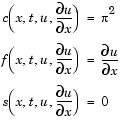
pdepe. See Introduction to PDE Problems for more information. For this example, the resulting equation is


pdepe can use. The function must be of the form
c, f, and s correspond to the  ,
,  , and
, and  terms. The code below computes
 c, f, and s for the example problem.


 and
and  of the boundary conditions in the function
 pdex1bc.
In the function pdex1bc, pl and ql correspond to the left boundary conditions ( ), and
 pr and qr correspond to the right boundary condition ( ).
).
 at which you want
 pdepe to evaluate the solution. Specify the points as vectors t and x.
t and x play different roles in the solver (see MATLAB Partial Differential Equation Solver). In particular, the cost and the accuracy of the solution depend strongly on the length of the vector x. However, the computation is much less sensitive to the values in the vector t.
This example requests the solution on the mesh produced by 20 equally spaced points from the spatial interval [0,1] and five values of t from the time interval [0,2].
pdepe with m = 0, the functions pdex1pde, pdex1ic, and pdex1bc, and the mesh defined by x and t at which pdepe is to evaluate the solution. The pdepe function returns the numerical solution in a three-dimensional array sol, where sol(i,j,k) approximates the kth component of the solution,  , evaluated at
 t(i) and x(j).
@ to pass pdex1pde, pdex1ic, and pdex1bc as function handles to pdepe.
Note
See the function_handle (@), func2str, and str2func reference pages, and the Function Handles chapter of "Programming and Data Types" in the MATLAB documentation for information about function handles.
|
 has only one component, but for illustrative purposes, the
example "extracts" it from the three-dimensional array. The surface plot
shows the behavior of the solution.
    u = sol(:,:,1);

    surf(x,t,u)
    title('Numerical solution computed with 20 mesh points')
    xlabel('Distance x')
    ylabel('Time t')
 , the final value of
  . In this example,

= t = 2. See "Evaluating the Solution at Specific Points" on
page 14-119 for more information.
Evaluating the Solution at Specific Points
After obtaining and plotting the solution above, you might be interested in a solution profile for a particular value of t, or the time changes of the solution at a particular point x. The kth column u(:,k) (of the solution extracted in step 7) contains the time history of the solution at x(k). The jth row u(j,:) contains the solution profile at t(j).
Using the vectors x and u(j,:), and the helper function pdeval, you can evaluate the solution u and its derivative  at any set of points
 xout
The example pdex3 uses pdeval to evaluate the derivative of the solution at xout = 0. See pdeval for details.
 | MATLAB Partial Differential Equation Solver | Changing PDE Integration Properties |  |