


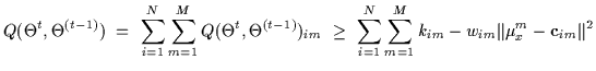
Each quadratic bound has a location parameter
![]() (a
centroid), a scale parameter wim (narrowness), and a peak value
at kim. The sum of quadratic bounds makes contact with the Qfunction at the old values of the model
(a
centroid), a scale parameter wim (narrowness), and a peak value
at kim. The sum of quadratic bounds makes contact with the Qfunction at the old values of the model
![]() where the gate
mean was originally
where the gate
mean was originally
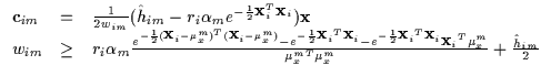
![]() and the covariance is
and the covariance is
![]() .
To facilitate the derivation, one may assume that
the previous mean was zero and the covariance was identity if the data
is appropriately whitened with respect to a given gate.
.
To facilitate the derivation, one may assume that
the previous mean was zero and the covariance was identity if the data
is appropriately whitened with respect to a given gate.
The parameters of each quadratic bound are solved by ensuring that it
contacts the corresponding Qim function at
![]() and
they have equal derivatives at contact (i.e. tangential
contact). Solving these constraints yields quadratic parameters for
each gate m and data point i in Equation 12
(kim is omitted for brevity).
and
they have equal derivatives at contact (i.e. tangential
contact). Solving these constraints yields quadratic parameters for
each gate m and data point i in Equation 12
(kim is omitted for brevity).
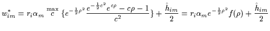
The tightest quadratic bound occurs when wim is minimal (without
violating the inequality). The expression for wim reduces to
finding the minimal value, wim*, as in
Equation 13 (here
![]() ). The f function is computed numerically only once and
stored as a lookup table (see Figure 2(a)). We thus
immediately compute the optimal wim* and the rest of the
quadratic bound's parameters obtaining bounds as in
Figure 2(b) where a Qim is lower bounded.
). The f function is computed numerically only once and
stored as a lookup table (see Figure 2(a)). We thus
immediately compute the optimal wim* and the rest of the
quadratic bound's parameters obtaining bounds as in
Figure 2(b) where a Qim is lower bounded.
The gate means ![]() are solved by maximizing the sum of the
are solved by maximizing the sum of the
![]() parabolas which bound Q. The update is
parabolas which bound Q. The update is
![]() .
This mean is
subsequently unwhitened to undo earlier data transformations.
.
This mean is
subsequently unwhitened to undo earlier data transformations.
![\begin{figure}\center
\begin{tabular}[b]{cccc}
\epsfxsize=1in
\epsfbox{mulut....
...
(c) $g$\space Function &
(d) Bound on $\Sigma_{xx}$ \end{tabular}
\end{figure}](img33.gif)