Mathematics

Simultaneous Linear Equations

Systems of simultaneous linear equations can be solved by two different classes of methods:

• Direct methods. These are usually variants of Gaussian elimination and are often expressed as matrix factorizations such as LU or Cholesky factorization. The algorithms involve access to the individual matrix elements.
• Iterative methods. Only an approximate solution is produced after a finite number of steps. The coefficient matrix is involved only indirectly, through a matrix-vector product or as the result of an abstract linear operator.

Direct Methods

Direct methods are usually faster and more generally applicable, if there is enough storage available to carry them out. Iterative methods are usually applicable to restricted cases of equations and depend upon properties like diagonal dominance or the existence of an underlying differential operator. Direct methods are implemented in the core of MATLAB and are made as efficient as possible for general classes of matrices. Iterative methods are usually implemented in MATLAB M-files and may make use of the direct solution of subproblems or preconditioners.

The usual way to access direct methods in MATLAB is not through the lu or chol functions, but rather with the matrix division operators / and \. If A is square, the result of X = A\B is the solution to the linear system A*X = B. If A is not square, then a least squares solution is computed.

If A is a square, full, or sparse matrix, then A\B has the same storage class as B. Its computation involves a choice among several algorithms:

• If A is triangular, perform a triangular solve for each column of B.
• If A is a permutation of a triangular matrix, permute it and perform a sparse triangular solve for each column of B.
• If A is symmetric or Hermitian and has positive real diagonal elements, find a symmetric minimum degree order p = symmmd(A), and attempt to compute the Cholesky factorization of A(p,p). If successful, finish with two sparse triangular solves for each column of B.
• Otherwise (if A is not triangular, or is not Hermitian with positive diagonal, or if Cholesky factorization fails), find a column minimum degree order p = colmmd(A). Compute the LU factorization with partial pivoting of A(:,p), and perform two triangular solves for each column of B.

For a square matrix, MATLAB tries these possibilities in order of increasing cost. The tests for triangularity and symmetry are relatively fast and, if successful, allow for faster computation and more efficient memory usage than the general purpose method.

For example, consider the sequence below.

• [L,U] = lu(A);
  y = L\b;
  x = U\y;
  

In this case, MATLAB uses triangular solves for both matrix divisions, since L is a permutation of a triangular matrix and U is triangular.

Using a Different Preordering.   If A is not triangular or a permutation of a triangular matrix, backslash (\) uses colmmd and symmmd to determine a minimum degree order. Use the function spparms to turn off the minimum degree preordering if you want to use a better preorder for a particular matrix.

If A is sparse and x = A\b can use LU factorization, you can use a column ordering other than colmmd to solve for x, as in the following example.

• spparms('autommd',0); 
  q = colamd(A);
  x = A (:,q) \ b;
  x(q) = x;
  spparms('autommd',1);
  

If A can be factorized using Cholesky factorization, then x = A\b can be computed efficiently using

• spparms('autommd',0);
  p = symamd(A);
  x = A(p,p) \ b(p);
  x (p) = x;
  spparms('autommd',1);
  

In the examples above, the spparms('autommd',0) statement turns the automatic colmmd or symmmd ordering off. The spparms('autommd',1) statement turns it back on, just in case you use A\b later without specifying an appropriate pre-ordering. spparms with no arguments reports the current settings of the sparse parameters.

Iterative Methods

Nine functions are available that implement iterative methods for sparse systems of simultaneous linear systems.

Functions for Iterative Methods for Sparse Systems  

Function	Method
bicg	Biconjugate gradient
bicgstab	Biconjugate gradient stabilized
cgs	Conjugate gradient squared
gmres	Generalized minimum residual
lsqr	LSQR implementation of Conjugate Gradients on the Normal Equations
minres	Minimum residual
pcg	Preconditioned conjugate gradient
qmr	Quasiminimal residual
symmlq	Symmetric LQ

These methods are designed to solve or . For the Preconditioned Conjugate Gradient method, pcg, A must be a symmetric, positive definite matrix. minres and symmlq can be used on symmetric indefinite matrices. For lsqr, the matrix need not be square. The other five can handle nonsymmetric, square matrices.

All nine methods can make use of preconditioners. The linear system

is replaced by the equivalent system

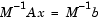
The preconditioner M is chosen to accelerate convergence of the iterative method. In many cases, the preconditioners occur naturally in the mathematical model. A partial differential equation with variable coefficients may be approximated by one with constant coefficients, for example. Incomplete matrix factorizations may be used in the absence of natural preconditioners.

The five-point finite difference approximation to Laplace's equation on a square, two-dimensional domain provides an example. The following statements use the preconditioned conjugate gradient method preconditioner M = R'*R, where R is the incomplete Cholesky factor of A.

• A = delsq(numgrid('S',50));
  b = ones(size(A,1),1);
  tol = 1.e-3;
  maxit = 10;
  R = cholinc(A,tol);
  [x,flag,err,iter,res] = pcg(A,b,tol,maxit,R',R);
  

Only four iterations are required to achieve the prescribed accuracy.

Background information on these iterative methods and incomplete factorizations is available in [2] and [7].

Factorization

Eigenvalues and Singular Values