Recognizing User's Context from Wearable Sensors: Baseline System
Brian Clarkson†,
Kenji Mase‡, and Alex Pentland†
We describe experiments in recognizing a person’s situation from only a wearable camera and microphone. The types of situations considered in these experiments are coarse locations (such as at work, in a subway or in a grocery store) and coarse events (such as in a conversation or walking down a busy street) that would require only global, non-attentional features to distinguish them.
Keywords: contextual computing, peripheral sensing, Hidden Markov Models, HMM, computer vision, computer audition, wearable computing
I.
Introduction
We describe a baseline system for training and classifying natural situations. It is a baseline system because it will provide the reference implementation of the context classifier against which we can compare more sophisticated machine learning techniques. It should be understood that this system is a precursor to a system for understanding all types of observable context not just location. We are less interested in obtaining high precision and recall rates than we are in obtaining appropriate model structures for doing higher order tasks like clustering and prediction on a user’s life activities.
II.
Background
There has been some excellent work on recognizing various kinds of user situations via wearable sensors. Starner [6] uses HMMs and omnidirectional and directional cameras to determine the user’s location in a building and current action during a physical game. Aoki also uses a head mounted directional camera to determine indoor location in [1]. Sumi et al. uses locational and history context to provide a wearable exhibition agent in [7]. Brand [2] presents an interesting idea for determining the states of human activity. His work relates strongly to the underlying motivation of this work (see author’s previous work in [3] [4]). Finally, Sawhney [5] provides an excellent example of the use of auditory context on a wearable messaging system.
III. Baseline System Outline
A wearable computer was constructed for the purposes of labeling a stream of audio/visual features with tags such as Entering Office, or Leaving Kitchen as the wearer went through his day. The classes were modeled with ergodic HMMs in the simplest way and used in a maximum likelihood classifier. The baseline system refers to this traditional and straightforward use of HMMs (see Figure 2).
The features we obtained from a wearable video camera and a wearable microphone are listed in Table 4. The camera was 1” x 1” x ½” pinhole CCD mounted to the chest strap. The microphone was a omnidirectional boundary microphone, also mounted to the chest strap. (see Table 1) The features together describe the 24 dimensional feature space in which HMMs were trained and tested. A wearable computer was used to allow the user to concurrently label events and locations as he experienced them. Of course, in general this is potentially disruptive to the user’s activities. However, for this experiment we tried to select classes that were not disturbed by the labeling action.
|
|
|
Table 1 The labeling wearable: (1) the touch sensitive pad for Unistroke input, (2) sensor package containing pinhole CCD and boundary microphone.
Also, we designed the actual interface to the labeling wearable so that it requires minimal use of one hand, no visual attention and limited auditory attention. The interface is a small handheld pad with 2 buttons, that allows the user to execute commands by drawing Unistroke characters on the pad with his thumb. Auditory feedback is provided via an earplug.
IV.
Contextual
Situations Considered
The situations that we have qualitatively considered so far are quite limited since they only involve entering and leaving 3 selected indoor locations:
1. Enter Office
2. Leave Office
3. Enter Kitchen
4. Leave Kitchen
5. Enter Black Couch Area (BCA)
6. Leave BCA
Many more are at this very moment being added to the database. Please see Figure 1 for a map of the area. The 3 boxes refer to the areas that were labeled whenever the user entered or left them. The path connecting these areas is not an actual path but just an estimation of the usual route that the user took to get between these 3 areas.
Other than the selection of the 3 areas for labeling, the conditions of this experiment were quite freeform. No effort was made to control for spontaneous situations since we wished to collect data under the most natural conditions possible.
· Natural movement and posture
· Spontaneous conversations in the hallway
· Constant shifting of the sensor package on the user’s body.
Basically, we want to emphasize that except for the user having a handheld device for labeling, all other conditions were kept as natural as possible. Of course, we shouldn’t ignore that the scenario was quite limited.
Figure 1: Location Map
The events 1-6 were labeled with impulses in time. For example when the user entered the kitchen, he marked the moment he passed through the doorway by pressing the label button on the handheld touch pad. See Table 2 for the number of labels collected for each event. For each of the events we partitioned the sets into separate training sets and testing sets.
|
Events |
# of Examples |
|
Leave Office |
31 |
|
Enter Office |
27 |
|
Leave BCA |
21 |
|
Enter BCA |
22 |
|
Leave Kitchen |
21 |
|
Enter Kitchen |
22 |
Table 2: The Data Set
V.
The
Models
The models used for determining the occurrence of events from the sensor stream were fully connected HMMs. We trained an HMM on each of the six events separately. Classification was achieved by using the Viterbi algorithm to obtain an estimate of the event likelihood for a window of features. If the likelihood exceeded a threshold then the event was triggered.
Figure 2 Overview of the Baseline System: 24 dimensional A/V features sampled at 5Hz enter the training pipeline at the left. HMMs are trained with varying numbers of states and window sizes. The HMMs that give maximum testing performance are selected.
To construct the training examples we took a time window of features around each of the impulse labels in the training set. This same window size was used in the Viterbi algorithm during classification. The window size represents the model’s use of context, so that larger window sizes mean more context is taken into account. Each state in the HMMs were constrained to have a single Gaussian. However, this still leaves the number of states and the window size undetermined.
We selected the parameters using brute force search over a range of state counts and window sizes. Using classification accuracy as the selection criterion we iterated over state counts from 1-10 and window sizes from 2-20 secs. See Figure 2 for a flow diagram of the training procedure just described and Figure 3 for an example of a criterion surface.
Figure 3 Accuracy vs. Free Model Parameters: this plot shows classification accuracy for the Enter Kitchen task for different HMM sizes and window sizes.
VI.
Results
We evaluated the models on a separate test set and obtained the following classification results. Since the thresholds for each model still needed to be determined we calculated Receiver-Operator Characteristic (ROC) curves for each model. The resulting curves are shown in Figure 4. We used the Equal Error Rate (EER) criterion (i.e. cost of false acceptance and of correct acceptance are the same) to choose optimal points on the ROC curves. Table 3 gives the resulting accuracies and the associated model parameters for each event.
|
Events |
# of States |
Window Size (secs) |
Accuracy (%) |
|
Leave Office |
8 |
20 |
85.8 |
|
Enter Office |
2 |
11 |
92.5 |
|
Leave BCA |
3 |
20 |
92.6 |
|
Enter BCA |
7 |
20 |
95.7 |
|
Leave Kitchen |
1 |
4 |
99.7 |
|
Enter Kitchen |
7 |
11 |
94.0 |
Table 3: The resulting model parameters and accuracies (based on EER) for each event/class.
The next plots (Figure 5Figure 6, Figure 7, and Figure 8) give the actual likelihood traces for the best and worst performing event models overlaid with the ground truth labels. Although in both cases the likelihood traces are quite noisy, the peak separation near actual labels is quite good (as supported by the ROC curves). Leave Kitchen (Figure 5) had the best performance with 99.7% accuracy achieved with just a 1 state HMM trained on 4 sec. feature windows. Leave Office (Figure 7) had the worst performance with 85.8% achieved with an 8 state HMM trained on 20 sec. feature windows. Notice that the window sizes exhibit themselves in the time resolution of the classifiers (Figure 6 and Figure 8).
These results are actually quite surprising (i.e. the high accuracy) considering the lack of context (perhaps in the form of a spatial grammar) and the coarse features. However, we can’t assume from these results that this method would work for a wide variety of conditions and events/situations. We still need to consider the possible degradation over time of the accuracy as the present situations drift away from their previously trained models. Basically we have no idea what the generalization properties of these models are.
Figure 4 Receiver-Operator Characteristic (ROC) Curves for each model when tested on the test set and varying the threshold on the likelihood.
Figure 5 Leave Kitchen Classification: This class achieved the best classification performance of all the classes and it used a 1 state HMM trained on 4 sec feature windows. This figure shows approx. 1 hr. of performance on the test set.
Figure 6 Leave Kitchen Classification (Zoom): This figure zooms in on a particular event in Figure 5. Notice the width of the likelihood spike is similar to the window size of this model (i.e. 4 secs).
Figure 7 Leave Office Classification: This class achieved the worst classification performance of all the classes and it used a 8 state HMM trained on 20 sec feature windows. This figure shows approx. 1 hr. of performance on the test set.
Figure 8 Leave Office Classification (Zoom): This figure zooms in on a particular event in Figure 7. Notice the width of the likelihood spike is similar to the window size of this model (i.e. 20 secs).
|
Figure 9 The Kitchen |
Figure 10 The Black Couch Area |
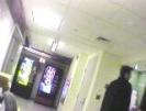
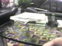

Figure 11 The Office
VII. Bibliography
1. Aoki, H., B. Schiele, and A. Pentland, Realtime Personal Positioning System for Wearable Computers. International Symposium on Wearable Computers '99, 1999.
2. Brand, M., Learning Concise Models of Human Activity from Ambient Video via a Structure-inducing M-step Estimator, . 1997.
3. Clarkson, B., K. Mase, and A. Pentland, The Familiar, . 1998: http://www.media.mit.edu/~clarkson/familiar/index.htm.
4. Clarkson, B. and A. Pentland, Unsupervised Clustering of Ambulatory Audio and Video, in ICASSP'99. 1999: http://www.media.mit.edu/~clarkson/icassp99/icassp99.html.
5. Sawhney, N., Contextual Awareness, Messaging and Communication in Nomadic Audio Environments, in Media Arts and Sciences. 1998, Massachusetts Institute of Technology.
6. Starner, T., B. Schiele, and A. Pentland. Visual Contextual Awareness in Wearable Computing. in Second International Symposium on Wearable Computers. 1998.
7. Sumi, Y., et al., C-MAP: Building a Context-Aware Mobile Assistant for Exhibition Tours, . 1998, ATR Media Integration & Communications Research Laboratories: Kyoto, Japan.
|
Modality |
Feature |
|
10 Filterbank Coeffs.
(10 dim.) |
|
|
Volume
(1 dim.) |
|
|
Last Speech Event
(1 dim.) |
|
|
Image Moments
(12 dim.) |
|
Table 4 Audio/Visual Features