Hard Constraints

Hard constraints represent absolute limitations imposed on the system. One example of a kinematic constraint is a skeletal joint. Our model instead follows the virtual work formulation [21]. In a virtual work formulation, all the links in a model have full range of unconstrained motion. Hard kinematic constraints on the system enforced by a special set of forces ${\bf c}$:

$$\ddot{{\bf q}} = {\bf W} \cdot ( {\bf Q} + {\bf c}({\bf q}, t) )$$ (4)

The formulas governing these constraints can be modified at run-time. It is essential that the constraint forces do not add energy to the system.

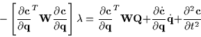
It can be shown that this requirement is satisfied if they are constructed so they lie in the null space complement of the constraint Jacobian:

$${\bf c}({\bf q}, t) = {\bf\lambda} \frac{\partial \dot{{\bf c}}}{\partial {\bf q}}$$ (5)

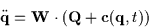
Combining that equation with the definition of the constraints results in a linear system of equations with only the one unknown, ${\bf \lambda}$:

$$-\left[ \frac{\partial {\bf c}}{\partial {\bf q}}^{T} {\b... ...}} \dot{\bf q} + \frac{\partial^{2} {\bf c}}{\partial t^{2}}$$ (6)

This equation can be rewritten to emphasize its linear nature. ${\bf J}$is the constraint Jacobian, ${\bf K}$ is a known constant vector, and ${\bf \lambda}$ is the vector of unknown Lagrange multipliers:

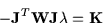$$- {\bf J}^{T} {\bf W} {\bf J} {\bf\lambda} = {\bf K}$$ (7)

Many fast, stable methods exist for solving equations of this form[15].